Josephood7

/* USER CODE BEGIN Header */
/**
  ******************************************************************************
  * @file           : main.c
  * @brief          : Main program body

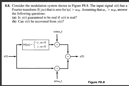
8.8. Consider the modulation system shown in Figure P8.8. The input signal$x(t)$has a Fourier transform$X(j\omega )$that is zero for$|\omega |>{\omega }^M$. Assuming that${\omega }^c>{\omega }^M$, answer the following questions: (a) Is$y(t)$guaranteed to be real if$x(t)$is real? (b) Can$x(t)$be recovered from$y(t)$? 

8.22. In Figure P8.22(a), a system is shown with input signal x(t) and output signal y() The input signal has the Fourier transform X(j) shown in Figure P8.22(b). Deter- mine and sketch Y(jo), the spectrum of y(1). x(t) y(t) -5w-3w 3w 5w -3w 3w ω cos(5wt) cos(3wt) Figure P8.22 632 Communication Systems Chap8 X(jo) -2w 2w Figure P8.22 Continued

8.41. In Problem 8.40, we introduced the concept of quadrature multiplexing, whereby two signals are summed after each has been modulated with carrier signals of iden- tical frequency, but with a phase difference of 90°. The corresponding discrete-time multiplexer and demultiplexer are shown in Figure P8.41. The signals xı[n] and x2[n] are both assumed to be band limited with maximum frequency wm, so that X;(ejw) = x2(ej“) = 0 for WM <w < 271 - wm. = = coswet H(jo) y(t) r(t) Demultiplexed outputs H(jw) y(t) sinct H(jw) -WM WM (b) Figure P8.40 Continued Coswon X,[n] r[n]=multiplexed signal X2[n] sinon (a) COS Hels) y, [n] r[n] Demultiplexed outputs H() y In] sinwon (b) Figure P8.41 040 (a) Determine the range of values for Wc so that xi[n] and x2[n] can be recovered from r[n]. (b) With we satisfying the conditions in part (a), determine H(ejw) so that yı[n] xi[n] and y2[n] x2[n].

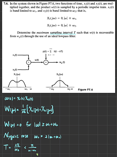
In the system shown in Figure P7.6, two functions of time, x_1(t) and x_2(t), are multiplied together and the product w(t) is sampled by a periodic impulse train. x_1(t) is band limited to omega_1, and x_2(t) is band limited to omega_2, that is, X_1(j omega) = 0, |omega| greaterthanorequalto omega_1, X_2(j omega) = 0, |omega| greaterthanorequal omega_2. Determine the maximum sampling interval T such that w(t) is recoverable from w_p(t) through the use of an ideal lowpass filter.

Shown in Figure P7.23 is a system in which the sampling signal is an impulse train with alternating sign. The Fourier transform of the input signal is as indicated in the figure. a) For< Tr/2m), sketch the Fourier transform of xp(t) and y(t). b For <Tr/(2M,determine a system that will recover xtfrom xpt. c For < T/2M),determine a system that will recover x(tfrom y(t. d) What is the maximum value of in relation to M for which x(t can be recov ered from either xp(t) or y(t)? p(t) xp(t) x(t) H(jw) y(t p(t) X(jw) UM H(jw) -3TT =T 3TT Figure P7.23

A signal limited in bandwidth to |omega| < W can be recovered from non-uniformly spaced samples as long as the average sample density is 2(W/2 pi) samples per second. Refer to the following figures and suppose x(t) is band-limited, i.e., X(j omega)) = 0 for |omega| > W; p(t) is the sampling impulse train; f(t) is a periodic waveform with period T = 2 pi/W. Since f(t) multiplies an impulse train, only its value f(0) = a and f(delta) = b are significant Hi(jo)) is a 90 degree phase shifter. Its frequency response is: H_1(j omega) = j for omega > 0 and H_1 (j omega) = - j for omega < 0 H_2(j omeag) is an ideal low pass filter. Its frequency response is: H_2(j omeag)) = K for 0 < omega < W; H_2(j omega) = K* for -W < omega < 0; and H_2(j omega) = 0 for |Omega| > W where K is a (possibly complex) constant Find the Fourier Transform of p(t), y_1(t), y_2(t), and y_3(t). You can specify the Fourier Transform of y_1(t), y_2(t), and y_3(t) over the range 0 < omega < W. Specify the values of a, b, and K as functions of A such that z(t) = x(t) for any band-limited x(t) and any A such that 0 < Delta < pi/W.

In this problem, we consider the discrete-time counterparts of the zero-order hold and first-order hold, which were discussed for continuous time in Sections 7 .1.2 and 7 .2. Let x[n] be a sequence to which discrete-time sampling, as illustrated in Figure 7.31, has been applied. Suppose the conditions of the discrete-time sampling theorem are satisfied; that is, ω_s> 2ω_M, where ω_sis the sampling frequency and

X(e^jω) = 0, ω_M≤ π. The original signal x[n] is then exactly recoverable from X_p[n] by ideal low pass filtering, which, as discussed in Section 7.5, corresponds to band-limited interpolation.

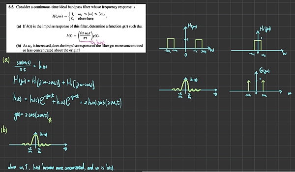
6.5. Consider a continuous-time ideal bandpass filter whose frequency response is H(ja)=10, elsewhere (a) If h(t) is the impulse response of this filter, determine a function g(t) such that h(r) - Sino,c (b) Asoc is increased, does the impulse response of the filter get more concentrated g(t). or less concentrated about the origin?

The straight-line approximation of the Bode magnitude plot of a causal and stable continuous-time LTI system is shown in Fig. 2. Questions: (1) Determine the frequency response of this system. (2) Make the Bode phase plot. 20 log10 (2) 94 dB 80 dB O dB/decade 120 dB/decade 40 dB/decade 12 dB 0.1 0.2 10 50 100 w (rad/sec) Figure

6.26. Consider an ideal highpass filter whose frequency response is specified as H(jw)# 1 0, otherwise (a) Determine the impulse response h(t) for this filter. (b) As oc is increased, does h(1) get more or less concentrated about the origin? (c) Determine s(0) and s(o0), where s(t) is the step response of the filter

Consider a system that consists of the cascade of two LTI systems whose frequency responses are given by 2 - e-jw Hi (ejw) = 1+ ke-jw? and 1 = H2 (ejw) = 1 - že-jw + je-j2w Find a difference equation describing the overall system. 

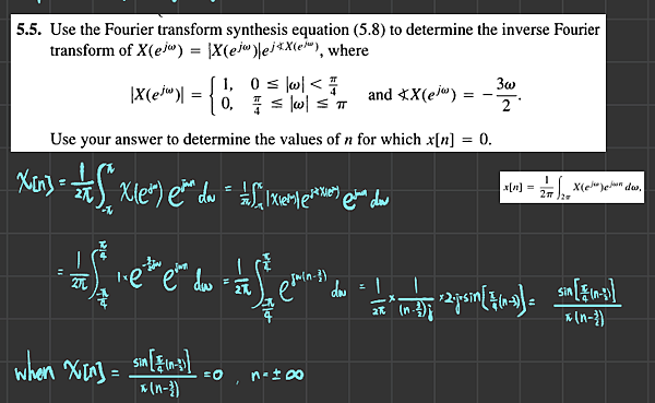
Use the Fourier transform synthesis equation (5.8) to determine the inverse Fourier 3W 2 and XX(e 0 Use your answer to determine the values of n for which x[n] = 0

Determine which, if any, of the following signals have Fourier transforms that satisfy each of the following conditions.

(a) Let$x[n]$be a discrete-time signal with Fourier transform$X\left(e^{j\omega }\right)$, which is illustrated in Figure P5.27. Sketch the Fourier transform of$w[n]=x[n]p[n]$for each of the following signals$p[n]$: (i)$p[n]=\cos \pi n$(ii)$p[n]=\cos (\pi n/2)$(iii)$p[n]=\sin (\pi n/2)$(iv)$p[n]={\sum }^{k=-\infty }\delta [n-2k]$(v)$p[n]={\sum }^{k=-\infty }\delta [n-4k]$g P5.27 The Discrete-Time Fourier Transform Chap. 5 (b) Suppose that the signal$w[n]$of part (a) is applied as the input to an LTI system with unit sample response$h[n]=\genfrac{}{}{0ex}{}{\sin (\pi n/2)}{\pi n}.$

A causal LTI system is described by the difference equation$y[n]=y[n-1]+y[n-2]+x[n-1]\text{. }$(a) Find the system function$H(z)=Y(z)/X(z)$for this system. Plot the poles and zeros of$H(z)$and indicate the region of convergence. (b) Find the unit sample response of the system. (c) You should have found the system to be unstable. Find a stable (noncausal) unit sample response that satisfies the difference equation.

(a) Consider a discrete-time system with unit sample response Min) = () un + 3 (?) un). Determine a linear constant-coefficient difference equation relating the in and output of the system. (b) Figure P5.51 depicts a block diagram implementation of a causal LTI system (i) Find a difference equation relating x[n] and y[n] for this system. (ii) What is the frequency response of the system? (iii) Determine the system's impulse response. xin N Fig P5.51

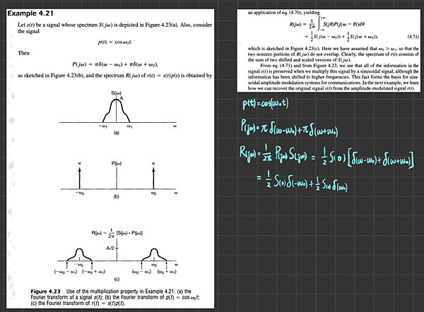
Let s(r) be a signal whose spectrum S(jo is depicted in Figure 4.23(a). Also, consider the signal p(t)-cos ω0. Then as sketched in Figure 4.23(b), and the spectrum R(jw) of t)-s()p)is obtained by S(jo) Plju) A/2 Figure 4.23 Use of the multiplication property in Example 4.21: (a) the Fourier transform of a signal s(t); (b) the Fourier transform of p(t)cos (c) the Fourier transform of r(t)-s(t)p(t).

Let us now consider r(t) as obtained in Example 4.21, and let 8(t) = r(t)pt), where, again, p(t) = cos wot. Then, R(jw), P(jw), and G(jw) are as shown in Figure 4.24. From Figure 4.24(c) and the linearity of the Fourier transform, we see that g(1) is the sum of (1/2)s(t) and a signal with a spectrum that is nonzero only at higher frequen- R(ja) A/2 WO WO (a) Pl) TT GO wu (b) G(jw) A/4 A/2 A/4 -200 2w (c) Figure 4.24 Spectra of signals considered in Example 4.22: (a) R(jw); (b) P(jw); (c) Gw). The Multiplication Property 325 cies (centered around +2wo). Suppose then that we apply the signal g(1) as the input to a frequency-selective lowpass filter with frequency response H(jw) that is constant at low frequencies (say, for w<wi) and zero at high frequencies (for 1>wi). Then the output of this system will have as its spectrum H(jw)G(jw), which, because of the particular choice of H(jw), will be a scaled replica of S(jw). Therefore, the output itself will be a scaled version of s(t). In Chapter 8, we expand significantly on this idea as we develop in detail the fundamentals of amplitude modulation.

another illustration of the usefulness of the Fourier transform multiplication

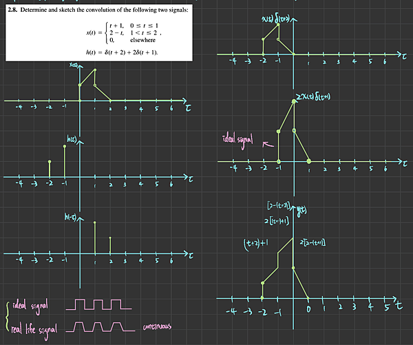
Determine and sketch the convolution of the following two signals: t +1, 0 <t<1 x(t) = {2-t, 1<t<2 0, elsewhere h(t) = (t + 2) + 2/(t+1)

Consider the cascade interconnection of three causal LTI system , illustrated in figure 3 , the impulse response h2[n] is h2[n] = delta[n] + delta [n-1] x[n] And the overall impulse response is shown bellow Find the impulse response h1,[n] Find the response of the overall system to the input x[n] = delta[n] - delta[n - 1]

how that if the response of an LTI system to an input x(t) is y(t), then the response to input x^'(t) = dx(t)/dt is y^'(t) = dy(t)fdt. Do this problem in two different ways (i) directly from the properties of linearity and time-invariance and the fact that x'(t) =lim_hrightarrow0 [x(t) - x(t-h))/h], and (ii) by differentiating the integral.

2.61. (a) In the circuit shown in Figure P2.61(a), x{t) is the input voltage. The voltage y(t) across the capacitor is considered to be the system output. L=1H m000000 y(t) C = 1F x(t) + (a) Figure P2.618 (i) Determine the differential equation relating X(t) and y(t). (ii) Show that the homogeneous solution of the differential equation from part (i) has the form Kjej@,! + Kzejw!. Specify the values of w, and w2. (iii) Show that, since the voltage and current are restricted to be real, the natural response of the system is sinusoidal. (b) In the circuit shown in Figure P2.61(b), x(t) is the input voltage. The voltage y(t) across the capacitor is considered to be the system output. ww R = 112 x(t) + y(t) C=1F (b) Figure P2.61b (i) Determine the differential equation relating x(t) and y(t). (ii) Show that the natural response of this system has the form Ke-", and spec- ify the value of a. (c) In the circuit shown in Figure P2.61(c), x(t) is the input voltage. The voltage y(t) across the capacitor is considered to be the system output. w R = 202 mm L = 1H x(t) TCF y(t) (c) Figure P2.610 (i) Determine the differential equation relating x(t) and y(t). (ii) Show that the homogeneous solution of the differential equation from part (i) has the form ef{Kjej21 + K2e j2}, and specify the value of a. (iii) Show that, since the voltage and current are restricted to be real, the natural response of the system is a decaying sinusoid.

2.45. (a) Show that if the response of an LTI system to x(t) is the output y(t), then the response of the system to x' (t) = dx(t) dt is y'(t). Do this problem in three different ways: (iii) By examining the system in Figure P2.45. x(t) u₁(t) h(t) y(t) Figure P2.45 b) Demonstrate the validity of the following relationships: (i) y'(t) = x(t) * h'(t) (ii) y(t) = (x(7) dT) * h'(t) = [',[x'(7) * h(7)]dt = x'(t) * ({ _'¸h(T)dt) [Hint: These are easily done using block diagrams as in (iii) of part (a) and the fact that u₁(t) * u_₁(t) = 8(t).]

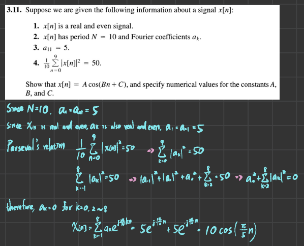
3.11. Suppose we are given the following information about a signal x[n]: 1. x[n] is a real and even signal. 2. x[n] has period N = 10 and Fourier coefficients ar. 3. Q11 = 5. 4. To Ślx[n]? = 50. n=0 A cos(Bn+C), and specify numerical values for the constants Show that x[n] = A cos(Bn+C), and specify numer B, and C.

3.16) Determine the output of the filter shown in Figure P3.16 for the following periodic je u inputs: (a) x1[n] = (-1)" (b) x2[n] = i + sin(n + ) (e) x3[n] = x.-(:)*4* u[n - 4k] 

Let x[n] be a periodic signal with period N = 8 and Fourier series coefficients ak = -ak-4. A signal y[n]) = (1+Q=1)")[n – 1) with period N = 8 is generated. Denoting the Fourier series coefficients of y[n] by bk, find a function f[k] such that bk = f[k]ak

Determine the Fourier series coefficients for each of the following discrete-time signals

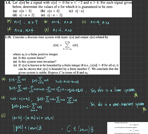
1.4. Let x[n] be a signal with x[n] = 0 for n < -2 and n > 4. For each signal given below, determine the values of n for which it is guaranteed to be zero. (a) xịn - 3] (b) x[n+ 4] (c) x[-n] (d) x[-n+2] (e) x[-n-2] 1.5.

1.18. Consider a discrete-time system with input x[n] and output y[n] related by yn] * x[k], k%3Dnールの where no is a finite positive integer. (a) Is this system linear? (a) Is this system time-invariant? (c) If x[n] is known to be bounded by a finite integer B (i.e., lx[n] < B for all n), it can be shown that y[n] is bounded by a finite number C. We conclude that the given system is stable. Express C in terms of B and no.

1.38. In this problem, we examine a few of the properties of the unit impulse function (a) Show that Hint: Examine δΔ(1). (See Figure 1.34.) (b) In Section 1.4, we defined the continuous-time unit impulse as the limit of the signal δΔ(t). More precisely, we defined several of the properties of δ(t) by examining the corresponding properties of δΔ(t). For example, since the signal Signals and Systems Chap. 1 converges to the unit step u(t) - lim ua(t), (P1.38-1) we could interpret δ(t) through the equation or by viewing δ(t) as the formal derivative of u(t) This type of discussion is important, as we are in effect trying to define 6(t) through its properties rather than by specifying its value for each t, which is not possible. In Chapter 2, we provide a very simple characterization of the behavior of the unit impulse that is extremely useful in the study of linear time- invariant systems. For the present, however, we concentrate on demonstrating that the important concept in using the unit impulse is to understand how it behaves. To do this, consider the six signals depicted in Figure P1.38. Show l(t) r2(t) -스 Δ2a

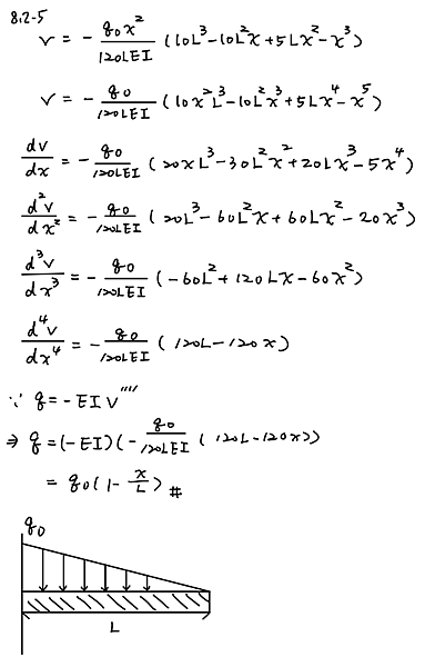
The deflection curve for a cantilever beam AB (see figure) is given by the following equation: upsilon (x) = - w_0 x^2/360L^2EI (45L^4 - 40 L^3x + 15 L^2x^2 - x^4) 

describe the load acting on the beam

Derive the equations of the deflection curve for a simple beam AB loaded by a couple Mo acting at distance a from the left-hand support (see figure) Also, determine the deflection δ0 at the point where the load is applied. Use the second-order differential equation of the deflection curve.

A cantilever beam has a length L = 3.6 m and a rectangular cross section (b = 400 mm, h = 600 mm). A linearly varying distributed load with peak intensity q₀ acts on the beam.

(a) Find peak intensity q₀ if the deflection at joint B is known to be 4.5 mm. Assume that modulus E = 205 GPa.

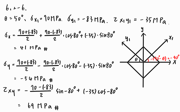
Two steel rods are welded together (see figure); the seam is oriented at angle θ = 50°. The stresses on the rotated element are σ_x1 = 70 MPa, σ_y1 = -83 MPa, and τ_x1y1 = -35 MPa. Find the state of plane stress on the element if it is rotated clockwise to align the _x1 axis with the longitudinal axis of the rods.

A shear wall in a reinforced concrete building is subjected to a vertical uniform load of intensity q and a horizontal force H, as shown in the first part of the figure. (The force H represents the effects of wind and earthquake loads.) As a consequence of these loads, the stresses at point A on the surface of the wall have the values shown in the second part of the figure (compressive stress equal to 8 MPa and shear stress equal to 3 MPa).

(a) Determine the principal stresses and show them on a sketch of a properly oriented element.

(b) Determine the maximum shear stresses and associated normal stresses and show them on a sketch of a properly oriented element.

The stresses acting on a stress element on the arm of a power excavator are ?x = 52 MPa and ?xy = 33 MPa. What

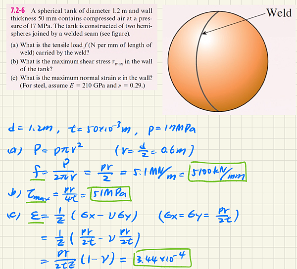
A spherical tank of diameter 1.2 m and wall thickness 50 mm contains compressed air at a pressure of 17 MPa. The tank is constructed of two hemispheres joined by a welded seam (see figure).

(a) What is the tensile load f (N per mm of length of weld) carried by the weld?

(b) What is the maximum shear stress τmax (Mpa) in the wallof the tank?

A pressurized steel tank is constructed with a helical weld that makes an angle α = 55°with the longitudinal axis (see figure). The tank has radius r = 0.6 m, wall thickness t = 18 mm, and internal pressure p = 2.8 MPa. Also, the steel has modulus of elasticity E = 200 GPa and Poisson’s ratio v = 0.30.

Determine the following quantities for the cylindrical part of the tank.